What is joint congruence?
Joint congruence is the measurement of two opposing joint surfaces as they relate to one another considering the 3D shape contour of each bone at their interface. For example, relating the femoral condyle to the tibial plateau or the temperomandibular condyle to the fossa.
Congruence analysis can result in:
- Analysis of the joint “gap” between the two opposing surfaces.
- Average shape representation of either joint surface.
- Computation of “normal” joint characteristics.
- Surgical indication for diseased or injured joints.
- Anthropologic study of joints.
- Forensic analysis by matching paired bones per individual or species.
How to perform joint congruence analysis
Analysis typically follows these steps:
- Select a set of CT scans of your intended specimen population.
- Place homologous landmark points on each specimen’s opposing joint surfaces
- Register and align all specimen landmark points
- Perform joint congruence analysis
Joint congruence analysis software
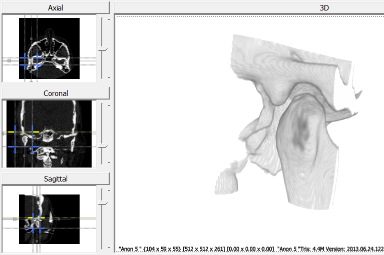
The following explains how to use a joint primitive to setup specimens for populations used in joint congruence using Stratovan Checkpoint. The example creates condyle and fossa specimens of the temporomandibular joint (TMJ) for their respective populations from a joint primitive. This tutorial includes:
- Loading a CT scan and using cropping to isolate a region of interest around the TMJ.
- Exporting the isolated condyle and fossa volume.
- Using right-to-left reflection for symmetry.
- Adding and adjusting the joint primitive.
- Adding the joint primitive’s patches to shape populations as specimens.
- Analyzing the matching specimens using joint congruence.
Load Scan and Export Volume
- Load a CT scan of a head. For this example, the scan includes both the fossa and condyle.
- Use the cropping lines to isolate the region of interest.
- In the export tab, click on “Export Volume” to save the cropped volume. To export the reflected volume, click on “Export Reflected Volume”.
Placing the Joint Primitive
- Load the exported volume.
- In the surface tab, select an iso value that produces surfaces without holes in the condyle and fossa.
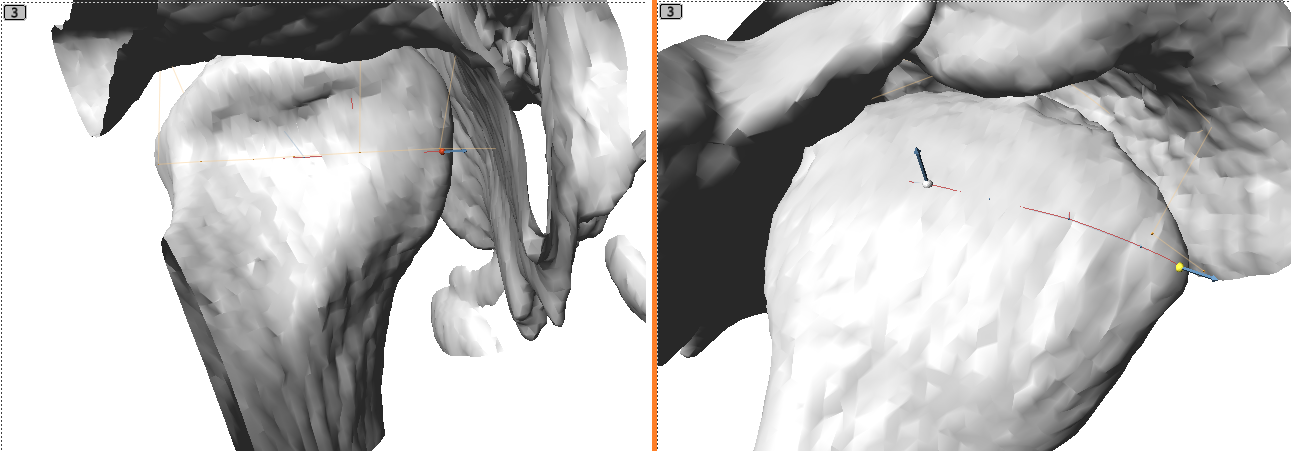
- Click the
 button, then hold ‘shift’ and left click on the condyle to add the joint primitive.
 - Move the red and yellow control points to the medial and lateral sides of the condyle.
- Optionally, to restrict the condyle white point to a plane that keeps this point equidistance from the lateral points, first, right click in the 3D or any slice window to bring up the pop menu and select “Align Avatar to:” -> “Joints” -> ‘Joint’. This aligns the avatar to the joint, placing it at the midpoint between the lateral red and yellow points and aligning the sagittal slice perpendicular to the lateral points. Next, right click on the joint’s overlay button and select the “Snap condyle white landmark to sagittal slice” command, which projects the condyle white point to the sagittal slice defined by the avatar and also selects the condyle white point. Finally, use the sagittal slice window to move the condyle white point.
Adjusting the Joint Primitive
- In the landmarks tab, select the joint primitive.
- Set the name and dimensions.
- Toggle the volume or surface with the
 or
or  buttons to verify that the top of the patch is on the top of the condyle. If the patch is upside down, then click the “Upside Down” button under “Direction”.
 - Use the “Flip” button to swap the point ordering, which is seen with the swapped yellow and red control point positions. This example places the yellow point on the lateral condyle position and the red point on the medial condyle position.
Adjusting Semi-Landmarks
- Rename the condyle patch under “Semi-landmark Group”.
- Drag the semi-landmark point in the slice window to adjust its position. The semi-landmark’s movement is restricted to the long dotted line.
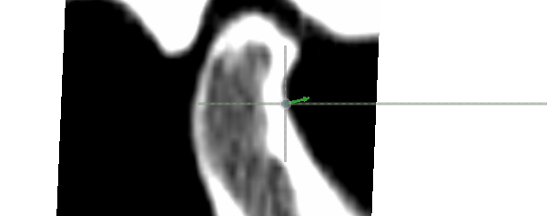
- Move to the next semi-landmark with the right arrow key on the keyboard or the “>” button under “Semi-landmark”. Toggle a semi-landmark as missing by selecting a slice window or 3D window and pressing the “M” key or by clicking the “Mark as ‘missing’” check box.
- Once all semi-landmarks in the condyle patch have been adjusted, click the “<” or “>” button under “Semi-landmark Group”, and repeat the above process for the fossa.
Create Populations and Add the Joint Primitive
- In the shape analysis tab, add two new populations, one named “5×5 Condyle Population” and a second named “5×5 Fossa Population”.
- Click the “+” button under the list of specimens to pop up the joint import window.
- Select the joint “TMJ” from the list. Name the specimen for each semi-landmark group.
- Select a population under “Import to Population” to import each of the specimens. Select the condyle population for the condyle semi-landmark group and the fossa population for the fossa semi-landmark group. Click “Ok” to import.
Joint Congruence Analysis
- After adding more joint primitives to the populations, the shape analysis can proceed. Select “Joint Congruence” under the “Analysis method”.
- Select the population to match with the “Matching Population”, then select the “5×5 Condyle Population” to match with the “5×5 Fossa Population”.
- Click “Edit Specimen Matching” to confirm the default matching or edit them. Click “Ok” to save the matches. These matches will remain even after closing Checkpoint or even after matching these specimens with another population’s specimens.
- Select a method for the analysis. Either “Average” or “Procrustes”, then click the “Analyze” button. The “Procrustes” method performs the generalized procrustes analysis.
Exporting Results
- Using the “Average” method for the analysis provides multiple results under “Result”, which can then be viewed and exported.
- To export a csv file with the landmarks of the rigidly aligned matching specimens, select “All” under “Result”, then select “CSV” under “Format”, and then click “Export”. Each row in the csv file lists the matched specimens with the name “Specimen A : Specimen B”, which is followed by the xyz landmark coordinates of “Specimen A” then the xyz landmark coordinates of “Specimen B”.
- To export a csv file with the distances between the matching landmarks of matching specimens, select “All Specimens Spacing” under “Result”, then select “CSV” under “Format”, and then click “Export”. Each row in the csv file lists the matched specimens with the name “Specimen A : Specimen B”, which is followed by the distances between the matched landmarks. The file identifies the matched landmarks used for each distance at the top of each column as “Mark A : Mark B”.